Math I Concepts Quiz
Math I
Unit-1.1 Set Theory
Set is a collection of well defined and distinct objects.
POINTS TO KNOW
- n(AᴜB) is the number of elements present in either of the sets A or B.
- n(A∩B) is the number of elements present in both the sets A and B.
FORMULAS
For two sets A and B
- n(AᴜB) = n(A) + (n(B) – n(A∩B)
For three sets A, B and C
- n(AᴜBᴜC) = n(A) + n(B) + n(C) – n(A∩B) – n(B∩C) – n(C∩A) + n(A∩B∩C)
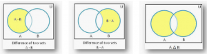
SOME VEEN DI AGRAM REPRESENTATIONS:
In above diagram set A is the subset of set B
Unit 1.2 Real Number
N FACT
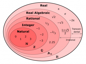
Nearly any number you can think of is a Real Number.
Real Numbers include:
- Whole Numbers (like 0, 1, 2, 3, 4, etc)
- Rational Numbers (like 3/4, 0.125, 0.333…, 1.1, etc )
- Irrational Numbers (like π, √2, etc )
Real Numbers can also be positive, negative or zero.
So what is NOT a Real Number?
- Imaginary Numbers like √−1 (the square root of minus 1) are not Real Number
- Infinity is not a Real Number
This diagram may help you to understand better:
Unit 1.3 Complex Number
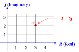
A complex number is any number which can be written as a+ib where a and b are real numbers and i=√−1 is an imaginary number.
a is the real part of the complex number and b is the imaginary part of the complex number.
Example for a complex number: 9 + i2

POINTS TO KNOW
- If the complex number a+ib=x+iy, then a=xand b=
- Fourth Roots of Unity, (1)1/4 are +1, -1, +i, -i
This may help you to identify real and imaginary numbers
Unit 2 Relation, Function and Graph
A rule which associates each element of the set (A) with at least one element in set (B).
Function:
A function is a relation between a set of inputs and a set of permissible outputs with the property that each input is related to exactly one output.
Eg:

A Condition for a Function:
Set A and Set B should be non-empty.
In a function, a particular input is given to get a particular output. So, A function f: A->B denotes that f is a function from A to B, where A is a domain and B is a co-domain.
- For an element, a, which belongs to A, aϵA, a unique element b, bϵB is there such that (a,b)ϵ f.
The unique element b to which f relates a, is denoted by f(a) and is called f of a, or the value of f at a, or the image of a under f.
- The range of f (image of a under f)
- It is the set of all values of f(x) taken together.
- Range of f = { y ϵ Y | y = f (x), for some x in X}
A real-valued function has either P or any one of its subsets as its range. Further, if its domain is also either P or a subset of P, it is called a real function.
Representation of Functions
Functions are generally represented as f(x)
Let , f(x)=x3
It is said as f of x is equal to x cube.
Functions can also be represented by g(), t(),… etc.
Domain & Range
The domain of a function f(x) is the set of all values for which the function is defined, and the range of the function is the set of all values that ff takes.

Here, Domain = {1,5,8}
Range = {a,b,c}
This will help you more:

Note: All ranges are co-domain but all co-domain are not range.
Types of functions
There are various types of functions in mathematics some of which are explained below in detail. The different functions types covered here are:
- One – one function (Injective function)
- Many – one function
- Onto – function (Surjective Function)
- Into – function
- Polynomial function
- Linear Function
- Quadratic Function
- Algebraic Functions
- Cubic Function
- Even and Odd Function
- Composite Function
- Constant Function
- Identity Function
One – one function (Injective function)
If each element in the domain of a function has a distinct image in the co-domain, the function is said to be one to one function.

For examples f: R R given by f(x) = 3x + 5 is one – one.
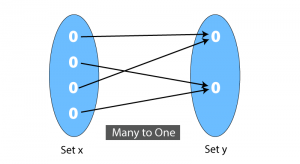
Many – one function
On the other hand, if there are at least two elements in the domain whose images are the same, the function is known as many to one function.
Onto – function (Surjective Function)
A function is called an onto function if each element in the co-domain has at least one pre-image in the domain.
Into – function
If there exists at least one element in the co-domain which is not an image of any element in the domain then the function will be Into function.
Linear Function
All functions in the form of ax + b where a, b∈R & a ≠ 0 are called as linear functions. The graph will be a straight line. In other words, a linear polynomial function is a first-degree polynomial where the input needs to be multiplied by m and added to c. It can be expressed by f(x) = mx + c.
For example, f(x) = 2x + 1 at x = 1
f(1) = 2.1 + 1 = 3
f(1) = 3
Cubic Function
A cubic polynomial function is a polynomial of degree three and can be expressed as;
F(x) = ax3 + bx2 + cx + d and a is not equal to zero.
Quadratic Function
All functions in the form of y = ax2 + bx + c where a, b, c∈R, a ≠ 0 will be known as Quadratic function.
Algebraic Functions
A function that consists of a finite number of terms involving powers and roots of independent variable x and fundamental operations such as addition, subtraction, multiplication, and division is known as an algebraic equation.
Even and Odd Function
If f(x) = f(-x) then the function will be even function & f(x) = -f(-x) then the function will be odd function
Example 1:
f(x) = x2sinx f(x) = -f(-x)
f(-x) = -x2sinx
it is odd function.
Example 2:
f(x)=x2 ⇒f(x)=f(−x) f(−x)=x2 it is even function.
Periodic Function
A function is said to be a periodic function if there exists a positive real numbers T such that f(u – t) = f(x) for all x ε Domain.
For example f(x) = sinx
f(x + 2π) = sin (x + 2π) = sinx fundamental
then period of sinx is 2π
Composite Function
Let A, B, C’ be three non-empty sets
Let f: A B & g : G C be two functions then gof : A C. This function is called composition of f and g
given g of (x) = g(f(x))
For example f(x) = x2 & g(x) = 2x
f(g(x)) = f(2x) = (2x)2 = 4x2
g(f(x)) = g(x2) = 2x2
Constant Function
The function f : P → P defined by b = f (x) = D, a ϵP, where D is a constant ϵ P, is a constant function.
- Domain of f = P
- Range of f = {D}
- Graph type: A straight line which is parallel to the x-axis.
In simple words, the polynomial of 0th degree where f(x) = f(0) = a0=c. Regardless of the input, the output always results in constant value. The graph for this is a horizontal line.

Identity Function
P= set of real numbers
The function f : P → P defined by b = f (a) = a for each a ϵ P is called the identity function.
- Domain of f = P
- Range of f = P
- Graph type: A straight line passing through the origin.
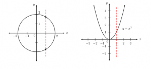
Vertical line test
Given the graph of a relation, there is a simple test for whether or not the relation is a function. This test is called the vertical line test. If it is possible to draw any vertical line (a line of constant \(x\)) which crosses the graph of the relation more than once, then the relation is not a function. If more than one intersection point exists, then the intersections correspond to multiple values of \(y\) for a single value of \(x\) (one-to-many).
- If any vertical line cuts the graph only once, then the relation is a function (one-to-one or many-to-one).
- The red vertical line cuts the circle twice and therefore the circle is not a function.
- The red vertical line only cuts the parabola once and therefore the parabola is a function.

Unit 3. Sequence and Series
Arithmetic Progression (AP)
- An arithmetic progression is a sequence of numbers in which each term after the first is obtained by adding a constant ‘d’ to the preceding term. The constant d is called the common difference.
- An arithmetic progression is given by a, (a + d), (a + 2d), (a + 3d), …
where a = the first term, d = the common difference
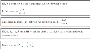
- If a, b, c are in AP then b = (a + c)/2
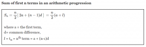
- nth term of an arithmetic progression
tn = a + (n – 1)d
where tn = nth term, a= the first term, d= common difference
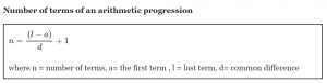
- Number of terms of an arithmetic progression
n=(l-a)/d+1
where n = number of terms, a= the first term , l = last term, d= common difference
FORMULAS
ADDITIONAL NOTES ON AP
To solve most of the problems related to AP, the terms can be conveniently taken as
3 terms: (a – d), a, (a +d)
4 terms: (a – 3d), (a – d), (a + d), (a +3d)
5 terms: (a – 2d), (a – d), a, (a + d), (a +2d)
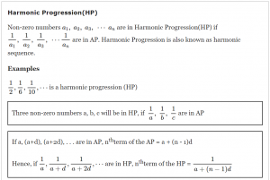
Harmonic Progression(HP)
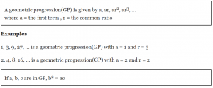
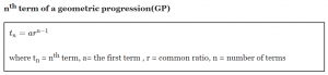
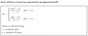
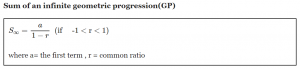
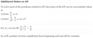
Geometric Progression (GP)
Geometric Progression (GP) is a sequence of non-zero numbers in which the ratio of any term and its preceding term is always constant.
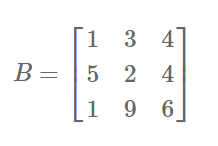
Unit 4: Matrix and Determinants
A matrix is simply a set of numbers arranged in a rectangular table.

There are several types of matrices, but the most commonly used are:
- Rows Matrix
- Columns Matrix
- Rectangular Matrix
- Square Matrix
- Diagonal Matrix
- Scalar Matrix
- Identity Matrix
- Triangular Matrix
- Null or Zero Matrix
- Transpose of a Matrix
Row Matrix:
A matrix is said to be a row matrix if it has only one row.

Column Matrix:
A matrix is said to be a column matrix if it has only one column.

Rectangular Matrix:
A matrix is said to be rectangular if the number of rows is not equal to the number of columns.

Square Matrix:
A matrix is said to be square if the number of rows is equal to the number of columns.
Diagonal Matrix:
A square matrix is said to be diagonal if at least one element of principal diagonal is non-zero and all the other elements are zero.

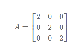
Scalar Matrix:
A diagonal matrix is said to be scalar if all of its diagonal elements are the same.
Identity or Unit Matrix:
A diagonal matrix is said to be identity if all of its diagonal elements are equal to one, denoted by I.

Triangular Matrix:
A square matrix is said to be triangular if all of its elements above the principal diagonal are zero (lower triangular matrix) or all of its elements below the principal diagonal are zero (upper triangular matrix).

Null or Zero Matrix:
A matrix is said to be a null or zero matrix if all of its elements are equal to zero. It is denoted by O.

Transpose of a Matrix:
Suppose A is a given matrix, then the matrix obtained by interchanging its rows into columns is called the transpose of A. It is denoted by At.
Determinants of a matrix
The determinant of a matrix is a special number that can be calculated from a square matrix.
For a 2×2 Matrix
For a 2×2 matrix (2 rows and 2 columns):


For a 3×3 Matrix
For a 3×3 matrix (3 rows and 3 columns):

Adjoint of a Matrix
Let A=[aij] be a square matrix of order n. The adjoint of matrix A is the transpose of the cofactor matrix of A. It is denoted by adj A. An adjoint matrix is also called an adjoint matrix.
Example:
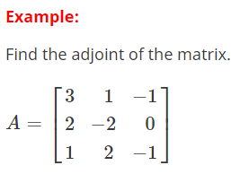
To find the adjoint of a matrix, first find the cofactor matrix of the given matrix. Then find the transpose of the cofactor matrix.

![]()
Inverse of a matrix
The inverse of A is A-1 only when:
A × A-1 = A-1 × A = I
Sometimes there is no inverse at all.
Formula:
Multiplication of a matrix

Unit 5: Analytical Geometry
Analytic Geometry is a branch of algebra that is used to model geometric objects – points, (straight) lines, and circles being the most basic of these. Analytic geometry is a great invention of Descartes and Fermat.
In plane analytic geometry, points are defined as ordered pairs of numbers, say, (x, y), while the straight lines are in turn defined as the sets of points that satisfy linear equations, see the excellent expositions by D. Pedoe or D. Brannan et al. From the view of analytic geometry, geometric axioms are derivable theorems. For example, for any two distinct points (x1, y1) and (x2, y2), there is a single line ax + by + c = 0 that passes through these points. Its coefficients a, b, c can be found (up to a constant factor) from the linear system of two equations
ax1 + by1 + c = 0
ax2 + by2 + c = 0,
Unit 6: Permutation and Combination
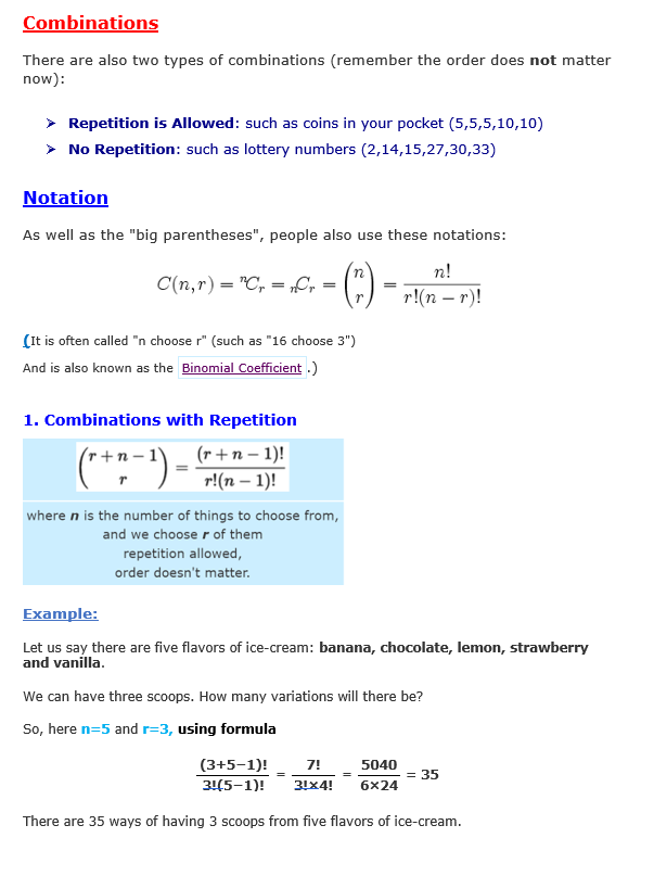
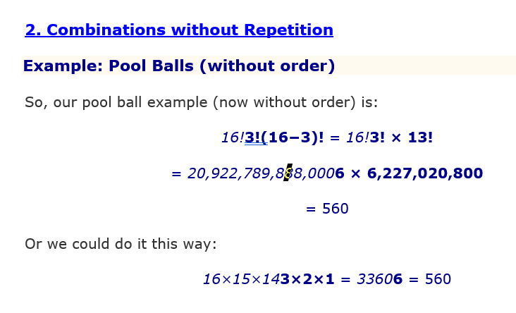
What’s the Difference?
- When the order doesn’t matter, it is a Combination.
- When the order doesmatter it is a Permutation.
In other words:
A Permutation is an ordered Combination.
Permutations
There are basically two types of permutation:
- Repetition is Allowed: It could be “333”.
- No Repetition: for example, the first three people in a running race. You can’t be first and
1. Permutations with Repetition
When a thing has n different types … we have n choices each time!
For example: choosing 3 of those things, the permutations are:
n × n × n(n multiplied 3 times)

Example: in the lock above, there are 10 numbers to choose from (0,1,2,3,4,5,6,7,8,9) and we choose 3 of them:
10 × 10 × 10 (3 times) = 103 = 1,000 permutations
So, the formula is simply:
| nr |
| where n is the number of things to choose from, and we choose r of them, repetition is allowed, and order matters. |
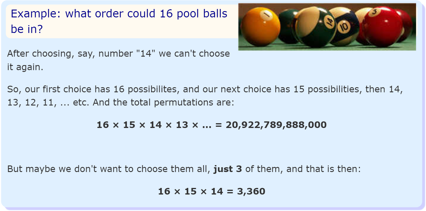
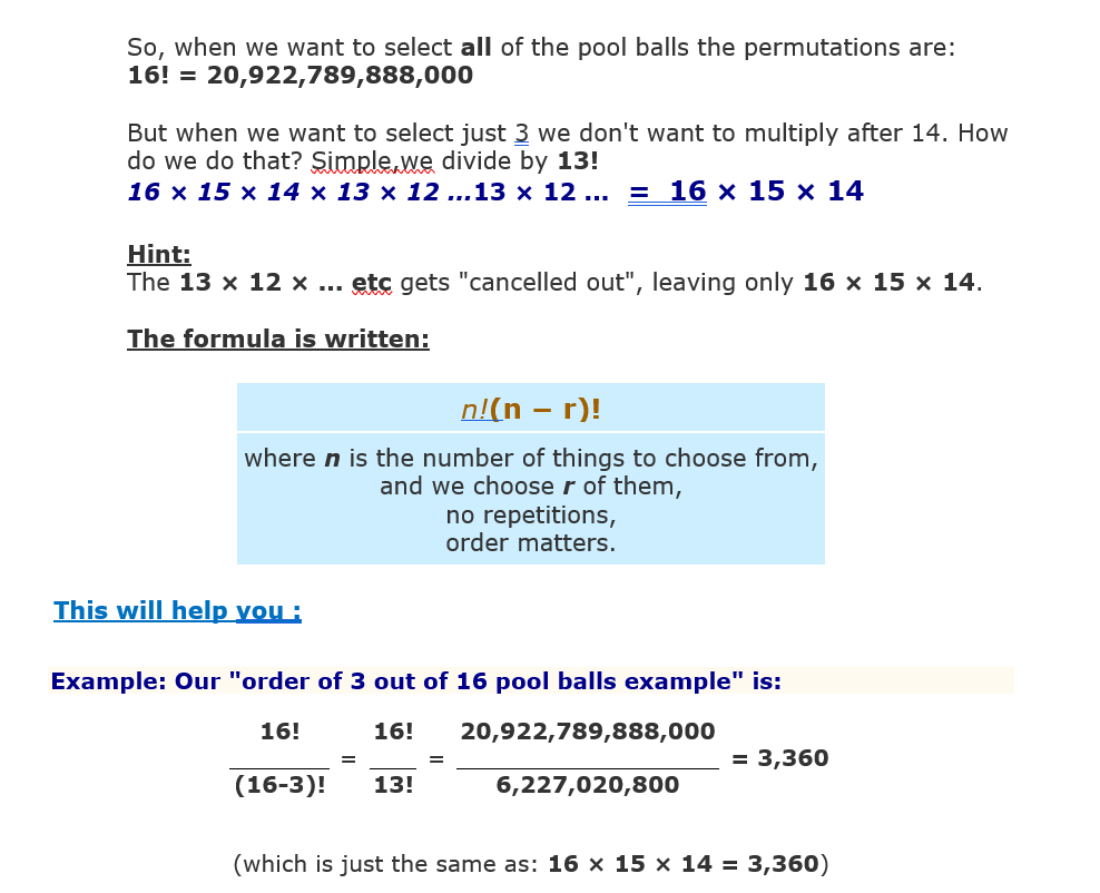
2. Permutations without Repetition
In this case, we have to reduce the number of available choices each time.
What’s the Difference?
- When the order doesn’t matter, it is a Combination.
- When the order doesmatter it is a Permutation.
In other words:
A Permutation is an ordered Combination.
Permutations
There are basically two types of permutation:
- Repetition is Allowed: It could be “333”.
- No Repetition: for example, the first three people in a running race. You can’t be first and
1. Permutations with Repetition
When a thing has n different types … we have n choices each time!
For example: choosing 3 of those things, the permutations are:
n × n × n(n multiplied 3 times)
Example: in the lock above, there are 10 numbers to choose from (0,1,2,3,4,5,6,7,8,9) and we choose 3 of them:
10 × 10 × 10 (3 times) = 103 = 1,000 permutations
So, the formula is simply:
| nr |
| where n is the number of things to choose from, and we choose r of them, repetition is allowed, and order matters. |
2. Permutations without Repetition
In this case, we have to reduce the number of available choices each time.

Syllabus
Course Title: Mathematics I (3 Cr.)
Course Code: CACS104
Year/Semester: I/I
Class Load: 5 Hrs. I Week (Theory: 3 Hrs., Tutorial: 1 Hr., Practical: 1 Hr.)
Course Description
This course includes several topics from algebra and analytical geometry such as set theory and real & complex number; relation, functions and graphs; sequence and series; matrices and determinants; permutation & combination; conic section and vector in space which are essential as mathematical foundation for computing.
Course Objectives
The general objective of this course is to provide the students with basic mathematical skills required to understand Computer Application Courses.
Course Contents
Unit 1 Set Theory and Real & Complex Number [7 Hrs.]
Concept, Notation and Specification of Sets, Types of Sets, Operations on Sets (Union, Intersection, Difference, Complement) and their Venn diagrams, Laws of Algebra of Sets (without proof), Cardinal Number of Set and Problems Related to Sets.
Real Number System, Intervals, Absolute Value of Real Number. Introduction of Complex Number, Geometrical Representation of Complex Number, Simple Algebraic Properties of Complex Numbers (Addition, Multiplication, Inverse, Absolute Value)
Unit 2 Relation, Functions and Graphs [8 Hrs.]
Ordered pairs, Cartesian product, Relation, Domain and Range of a relation, Inverse of a relation; Types of relations: reflective, symmetric, transitive, and equivalence relations. Definition of function, Domain and Range of a function, Inverse function, Special functions (Identity, Constant), Algebraic (linear, Quadratic, Cubic).
Trigonometric and their graphs. Definition of exponential and logarithmic functions, Composite function, (Mathematica)
Unit 3 Sequence and Series [7 Hrs.]
Sequence and – Series (Arithmetic, Geometric, Harmonic), Properties of Arithmetic, Geometric, Harmonic sequences, A. M., G. M., and H. M. and relation among them. Sum of Infinite Geometric Series. Taylor’s Theorem (without proof), Taylor’s series, Exponential series.
Unit 4 Matrices and Determinants [8 Hrs.]
Introductions of Matrices, Types of Matrices, Equality of Matrices, Algebra of Matrices, Determinant, Transpose, Minors and Cofactors of Matrix. Properties of determinants (without proof), Singular and non-singular matrix, adjoin and inverse of matrices Linear transformations, orthogonal transformations; rank of matrices. (MATLAB)
Unit 5 Analytical Geometry [8 Hrs.]
Conic Sections: Definitions (Circle, Parabola, Ellipse, Hyperbola and Related Terms), Examples to Explain the Defined Terms, Equations and Graphs of The Conic Sections Defined Above, Classifying the Defined Conic Sections by Eccentricity and Related Problems, Polar Equations of Lines, Circles, Ellipse, Parabolas, and Hyperbolas. (Mathematica / MATLAB)
Vectors in Space: Vectors in Space, Algebra of Vectors in Space, Length, Distance Between Two Points, Unit Vector, Null Vector. Scalar Product, Cross Product of Two and Three Vectors and Their Geometrical Interpretations and Related Examples. (MATLAB)
Unit 6 Permutation and Combination [7 Hrs.]
Basic Principle of Counting, Permutation of a. Set of Objects All Different b. Set of Objects Not All Different c. Circular Arrangement d.. Repeated Use of The Same Object. Combination of Things All Different, Properties of Combination.
Laboratory Works
Mathematica and/ or MATLAB should be used for above mentioned topics.
Teaching Methods
The general teaching pedagogy includes class lectures, group works, case studies, guest lectures, research work, project work, assignments (theoretical and practical), tutorials and examinations (written and verbal). The teaching faculty will determine the choice of teaching pedagogy as per the need of the topics.
Evaluation

Text Book
1. Thomas, G. B, Finney, R. S., “Calculus with Analytic Geometry”, Addison -Wesley, 9th Edition.
Reference Books
– Bajracharya D. R., Shreshtha, R. M. & et al, “Basic Mathematics I, II” Sukunda Pustak Bhawan, Nepal
– Budnick, F. S., “Applied Mathematics for Business, Economics and the Social Sciences”, McGraw-Hill Ryerson Limited.
– Monga, G. S., “Mathematics for Management and Economics”, Vikas Publishing House Pvt. Ltd., New Delhi.
– Paudel, K. C., GC. F. B., and et. al, “Higher Secondary Mathematics”, Asmita Publication & Distributors Pvt. Ltd, Nepal.
– Upadhayay, H. P., Paudel, K.0 & ct al, “Elements of Business Mathematics”, Pinnacle Publication.
– Yamane, T. “Mathematics for Economist”, Prentice-hall of India.


No comments:
Post a Comment